Blind source separation using Picard and Picard-O¶

The example runs the Picard algorithm proposed in:

Pierre Ablin, Jean-Francois Cardoso, Alexandre Gramfort “Faster independent component analysis by preconditioning with Hessian approximations” IEEE Transactions on Signal Processing, 2018 https://arxiv.org/abs/1706.08171

and Picard-O algorithm proposed in:

Pierre Ablin, Jean-François Cardoso, Alexandre Gramfort “Faster ICA under orthogonal constraint” ICASSP, 2018 https://arxiv.org/abs/1711.10873

# Author: Pierre Ablin <pierre.ablin@inria.fr>
#         Alexandre Gramfort <alexandre.gramfort@inria.fr>
# License: BSD 3 clause

import numpy as np
import matplotlib.pyplot as plt

from picard import picard

print(__doc__)

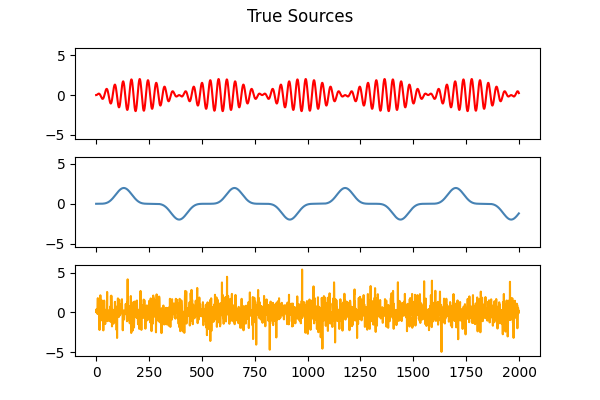
Generate sample data

np.random.seed(0)
n_samples = 2000
time = np.linspace(0, 8, n_samples)

s1 = np.sin(2 * time) * np.sin(40 * time)
s2 = np.sin(3 * time) ** 5
s3 = np.random.laplace(size=s1.shape)

S = np.c_[s1, s2, s3].T

S /= S.std(axis=1)[:, np.newaxis]  # Standardize data
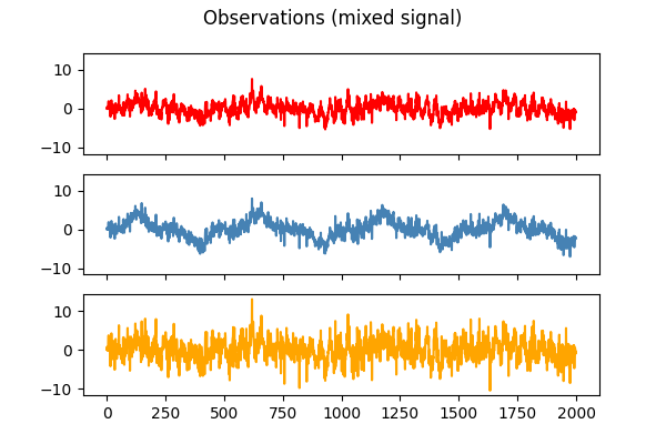
# Mix data
A = np.array([[1, 1, 1], [0.5, 2, 1.0], [1.5, 1.0, 2.0]])  # Mixing matrix
X = np.dot(A, S)  # Generate observations

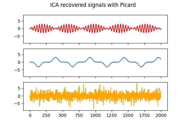
# Compute ICA
_, _, Y_picard = picard(X, ortho=False, random_state=0)
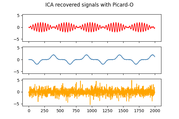
_, _, Y_picardo = picard(X, ortho=True, random_state=0)

Plot results

models = [X, S, Y_picard, Y_picardo]
names = ['Observations (mixed signal)',
         'True Sources',
         'ICA recovered signals with Picard',
         'ICA recovered signals with Picard-O']
colors = ['red', 'steelblue', 'orange']

for ii, (model, name) in enumerate(zip(models, names), 1):
    fig, axes = plt.subplots(3, 1, figsize=(6, 4), sharex=True, sharey=True)
    plt.suptitle(name)
    for ax, sig, color in zip(axes, model, colors):
        ax.plot(sig, color=color)

plt.show()

Total running time of the script: ( 0 minutes 0.615 seconds)

Gallery generated by Sphinx-Gallery